Project4: Stitching Photo Mosaics

A. IMAGE WARPING and MOSAICING

Goal:

Shoot and digitize pictures
Recover homographies
Warp the images
Blend images into a mosaic

1. Shoot the Pictures

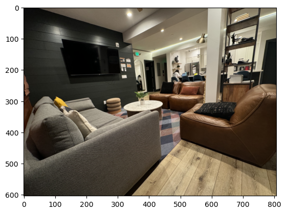
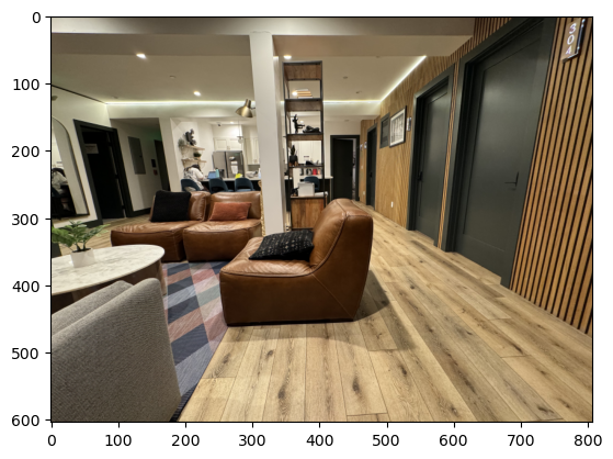
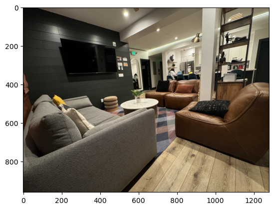
I shot pictures from my iPhone using a wide angle lenses.

1.2

1.1

2. Compute Homography matrix

In order to do the Homographies, we computer p' = Hp as following,

\begin{matrix} \begin{matrix} H = [\begin{matrix} h_{11} & h_{12} & h_{13} \\ h_{21} & h_{22} & h_{23} \\ h_{31} & h_{32} & h_{33} \end{matrix}] \end{matrix} \end{matrix}

\begin{matrix} {\begin{cases} x' i = \frac{h 11 x_{i} + h_{12} y_{i} + h_{13}}{h_{31} x_{i} + h_{32} y_{i} + h_{33}} \\ y' i = \frac{h 21 x_{i} + h_{22} y_{i} + h_{23}}{h_{31} x_{i} + h_{32} y_{i} + h_{33}} \end{cases} \end{matrix}

\begin{aligned} x'_{i} (h_{31} x_{i} + h_{32} y_{i} + 1) & = h_{11} x_{i} + h_{12} y_{i} + h_{13} \\ y'_{i} (h_{31} x_{i} + h_{32} y_{i} + 1) & = h_{21} x_{i} + h_{22} y_{i} + h_{23} \end{aligned}

\begin{aligned} h_{11} x_{i} + h_{12} y_{i} + h_{13} - h_{31} x'_{i} x_{i} - h_{32} x'_{i} y_{i} - x' i & = 0 \\ h_{21} x_{i} + h_{22} y_{i} + h_{23} - h_{31} y'_{i} x_{i} - h_{32} y'_{i} y_{i} - y'_{i} & = 0 \end{aligned},

Which could be represent to,

h * A_{i} - b = 0

Where

\begin{matrix} h = [h_{11}, h_{12}, h_{13}, h_{21}, h_{22}, h_{23}, h_{31}, h_{32}]^{T} \end{matrix}

\begin{matrix} \begin{matrix} A_{i} = [\begin{matrix} x_{i} & y_{i} & 1 & 0 & 0 & 0 & - x'_{i} x_{i} & - x'_{i} y_{i} \\ 0 & 0 & 0 & x_{i} & y_{i} & 1 & - y'_{i} x_{i} & - y'_{i} y_{i} \end{matrix}] \end{matrix} \end{matrix}

For n point correspondences, A will be a 2n * 8 matrix, and b will be a 2n * 1 vector. When n > 4 , the system is overdetermined which should be solved using least-squares (np.linalg.svd(A)).

3. Warp image

To avoid May result in gaps (“holes”) in the destination image because not every pixel in the destination image receives a value, use Inverse Warping.

For each pixel p'p $H^{-1}$ .
Apply H to the four corners of the source image to see where they map in the destination image.
$\mathbf{p}{\prime} = [x{\prime}, y{\prime}, 1]^T$ $\mathbf{p} = H^{-1} \mathbf{p}{\prime}$ . Then Normalize. Since x and y may not be integers, use interpolation to estimate the pixel values.
Computer alpha mask which determines the effective value‘s range.

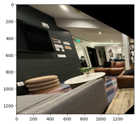
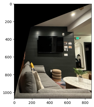
Warp the left image and we get:

2.1

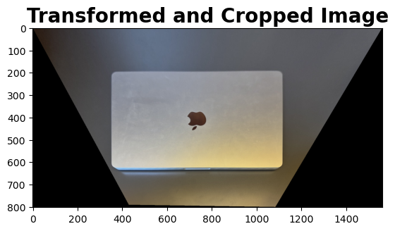
4. Image Rectification

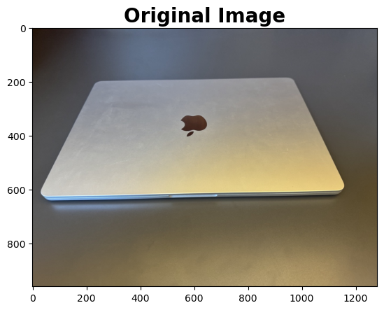
Then, use some photoes to test if warping function is right.

3.1

3.2

3.3

3.4

5. Blend the images into a mosaic

Image Registration: Aligning images so that corresponding points match. This involves finding the transformation (homography) that maps points from one image to another.
Image Warping: Applying the computed homography to warp images into a common coordinate frame.
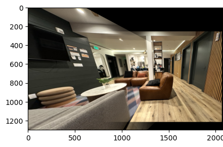
Blending: Combining the warped images into a single image, minimizing visible seams and artifacts.

The original photoes show as follow:

1.2

1.1

The warped left photo show as follow:

2.1

Mosaic image:

78a31fac-4bd3-477e-95b7-3b2cc6d834af

B. FEATURE MATCHING for AUTOSTITCHING

1. Detecting Corner Features

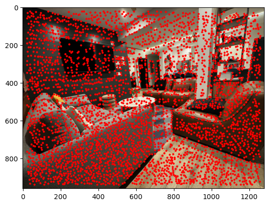
Using the provided Harris corner detector, I identified the corner features. To reduce the number of detected corners, I set the minimum distance between corners to 5 pixels and discarded 20 pixels along the edges. The result is displayed below:

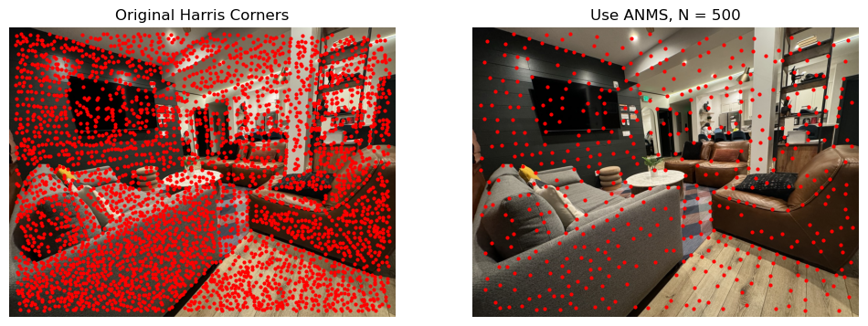
Next, Implemented the Adaptive Non-Maximal Suppression (ANMS) algorithm to select a fixed number of the best corners that are well-distributed spatially.

• For each corner x_i , find the distance r_i to the closest corner that has a stronger response.

\begin{matrix} (1) & r_{i} = min_{x_{j} \in {S | f (x_{j}) > f (x_{i})}} ∥ x_{i} - x_{j} ∥, where c = 0.9 \end{matrix}

Here, S is the set of all corners with a stronger response than corner x_i , and c is a robustness parameter as described in the paper.

• Sort these distances r_i in descending order and select the top N corners.

2. Extracting Descriptors

Based on Corner Strength : In interest point detection, the corner strength is the metric that determines the “importance” of each interest point. The ANMS strategy suppresses points based on the corner strength of each interest point.

Suppression Strategy: We use a “suppression radius” to define the neighborhood size. Within this neighborhood, only the interest point that is the maximum within radius will be retained.

Gradually Expanding Radius: Conceptually, we begin with and then incrementally increase until we reach the desired number of interest points .

Global Maximum: The first element in the list is the global maximum, which is never suppressed regardless of the radius. As the suppression radius decreases from infinity, new interest points are added to the list. Once an interest point is added, it remains in the list because a point that is the maximum at a certain radius will continue to be the maximum at any smaller radius.

3. Matching Descriptors

Identifying Feature Points of the Same Object or Position in Images: Feature descriptors are used to represent the pixels around a specific location in an image.

Lowering Sampling Frequency: For each interest point, we sample an 8 × 8 pixel block around its sub-pixel location with a sampling interval of 5 pixels. In the illustration, sampling around each feature point at 5-pixel intervals minimizes the effect of positional error on the descriptor.

Avoiding Aliasing: Sampling is done at a higher pyramid level than the detection scale to ensure a sampling rate of approximately once per pixel. Let s=5.

Normalization of the Descriptor Vector: After sampling, the descriptor vector is normalized to have a mean of 0 and a standard deviation of 1, ensuring invariance of features to affine changes in intensity (offset and gain).

Haar Wavelet Transformation: Finally, an 8 × 8 descriptor block undergoes a Haar wavelet transform, forming a 64-dimensional descriptor vector of wavelet coefficients . Due to the orthogonality of the Haar wavelet, Euclidean distances between features are preserved under this transformation.
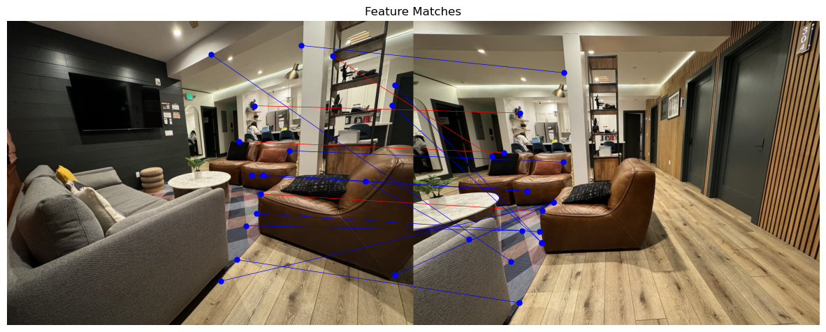
The result is displayed below:

4. Compute Homography Using RANSAC

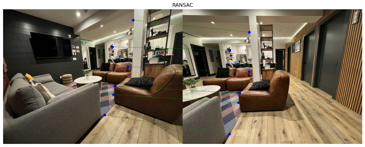
To compute homography using RANSAC, we iteratively select a minimal subset of point correspondences (typically 4) to estimate the homography matrix. For each subset, we calculate the homography and evaluate how well it aligns all points by counting inliers—points that fall within a specified distance threshold when transformed. This process is repeated over many iterations to maximize inliers, thus refining the homography estimation by prioritizing matches that align most accurately while excluding outliers. The final homography is derived from the subset with the most inliers, providing a robust transformation despite the presence of mismatches.

The result is displayed below:

5. Produce a mosaic

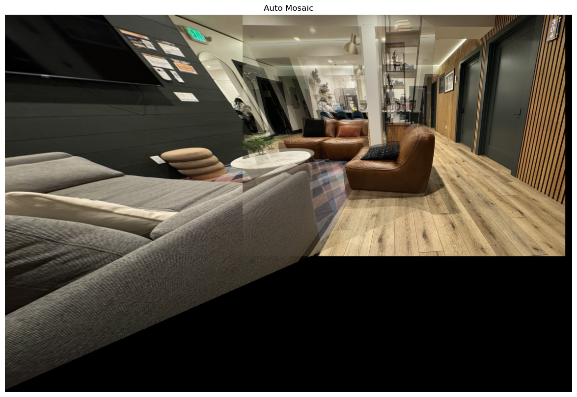
Last, we mosaic the two images. The result with Hand-Annotated H and Automatically H is displayed below:

78a31fac-4bd3-477e-95b7-3b2cc6d834af

Learned

In Project 4, I learned how to create seamless photo mosaics using homography-based transformations.

Capturing images with sufficient overlap was key to aligning them effectively. Calculating homographies taught me to map points between images, especially using least-squares for overdetermined systems. Inverse warping minimized gaps by mapping destination pixels back to the source, and interpolation ensured smooth transitions. Using the Harris corner detector with ANMS helped identify well-distributed, strong feature points, while extracting descriptors with reduced sampling frequency and normalization enhanced robustness to intensity variations. Implementing RANSAC allowed me to refine homographies by excluding outliers, yielding stable transformations.

Finally, blending techniques were crucial to produce a seamless mosaic by aligning images with minimized visible seams. This project deepened my understanding of image processing, feature matching, and transformation techniques fundamental to computer vision.